How does light intensity influence photosynthesis in Egeria densa

During one week, we, students at the FDV Bachelor program, designed an interdisciplinary scientific project aiming at comparing a biological sensor with an electronic one. We decided to work with Egeria densa, an algae mostly used in aquarium and that releases a lot of oxygen (O2) while doing photosynthesis.

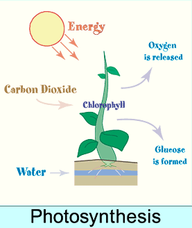
Photosynthesis is a process by which plants form glucose and release O2 using the energy from the sun, water and carbon dioxide (CO2). For more explanations about the photosynthesis process, you can have a look at this video.

In this project, we wanted to see if Egeria densa can be used to measure the intensity of light, regarding how much O2 is released by the algae while doing photosynthesis. We wanted to compare the range, accuracy and precision of the two different sensors. The accuracy of a sensor is how far is the measured value from the true value. The precision is how far are the measured values apart from one another. The range is the limits between which the sensor will be able to measure values.

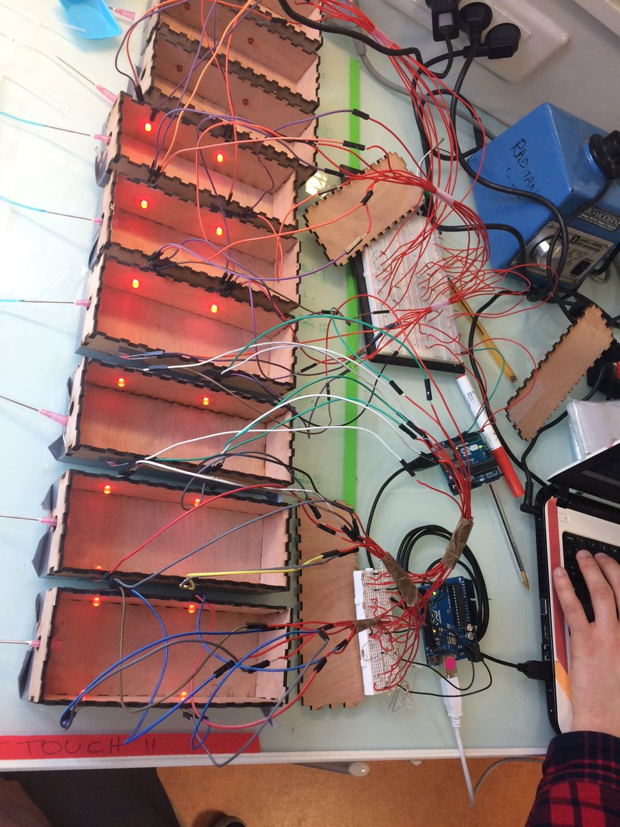
First, we designed closed wood boxes with holes for the LEDs, in order to have a good control on light intensity exposure. It looked like this :

To do so, we create a protocol in which Egeria densa were put in a syringe with tap water, connected to a clear rubber tube full of ink. When O2 was released by the algae, the ink was moving out of the tube. We also build a device (a box) that blocks noisy emissions of light, and emits a red beam at a certain intensity. Thanks to that, we were able to measure how much O2 was released, and by consequence, to measure the impact of the LED intensity on photosynthesis.

Here are the graphs we obtained :

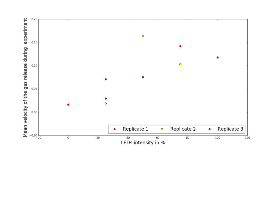
As we can see on those graphs, there are no obvious trend, even though we can draw some observations.

However, we can see that for the biological sensor, the negative control (0%) and the 25% intensity curves have kind of the same trend, therefore, we can think that the sensor doesn’t sense any changes between 0% and 25%. The same thing between the positive control (100%) and the 75% intensity curves. With those observations, we can say that probably, the range of the biological device is something like 25%-75%, where 75% is the saturation point.

The response time of the biological sensor, we can assume regarding our graphs that it takes approximately an hour for the sensor to have a constant value. This is explained by the fact that the algae has to adapt to the new LED intensity.

As for the response time of the electronic sensor, we measured it at 200ms. Indeed, we took measurements every 100 ms and only the third value was constant. Therefore, we had to wait for 2 values, meaning 100ms x 2 which equal to 200ms, our response time.

To conclude, we cannot really conclude with a statistical approach with the results we got.

Maybe one way to improve our experiment and to have more relevant results would be to use O2 probes, instead of the rubber tube. We could also design another box that is darker, and more easy to adapt and use for the large audience. It could become an interdisciplinary tool to understand that a sensor can be very surprising and innovative.

We also imagine using another organism, such as a bacteria that produces gas, or an enzyme.

For more informations about the ‘Photosynthetic strategies of Egeria densa”, please read this article.

Photosynthesis pictures is from : http://www.factmonster.com/ipka/A0775714.html

Here is our storify : https://t.co/gPgQCCfJzH 

Here is an identity card of our organism : Fiche - Egeria-Densa-Sr.pdf. Accessed January 20, 2017.
http://www.centrederessources-loirenature.com/mediatheque/especes_inva/fiches_FCBN/Fiche%20-%20egeria-densa-sr.pdf 

Thanks for reading ! See you soon !

Mimosa Action & Humidity's impact on its reaction to touch

Mimosa Action!

Hi there ! We are students from the “Frontiers of Life” bachelor, created and hosted by the Centre of Research and Interdisciplinarity ! The Biosensors seminary has slowly come to an end, and the project we worked on and are about to present, is the last one out of 4.

For those who do not know what the Biosensors are and missed our first blog posts, it’s an interdisciplinary seminar during which we develop and design in small groups several one-week scientific research-projects connected to each other by various notions such as light, forces and chemical gradients.

The aim of these projects is to observe and compare biological (plants, bacteria, insects, vertebrate, human ….) and electronic sensors (light, movement, conductivity, temperature sensors…).

This week, the comparison wasn't necessary, and we were free to develop any project, as long as it involved sensing (biological or electrical).

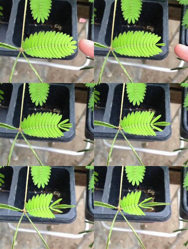
For our last project, we decided to study one of the most fascinating phenomena in the plant kingdom : thigmonasty. Thigmonasty consists in the response of a plant to touch or vibrations.  Mimosa pudica appears in scientific literature as a common example capable of responding to various stimuli (rain drops, wind …)

We got inspired by a project that had been conducted by former FDV students in 2013, named “Electrical response of Mimosa pudica to an external stimulus”. Mimosa pudica is a herb that has leaves that fold inward when touched. The project consisted in comparing the voltage response of Mimosa pudica  (in terms of electrical potential) according to the nature of the stimulus. They could observe that the response differs whether the stimulus was mechanical or electronic.

After more bibliographic research, we realised that water was the basis of the thigmonastic reaction.

Indeed, the thigmonastic movement is produced by the main pulvinus (sort of articular surface from a plant) at the base of the petiole (stalk that attaches the leaf to the stem) and «results from the explosive loss of water from specific cells in the pulvini, causing the cells temporarily to collapse and inducing very quick curvature in the organ where they are located»

(http://plantsinaction.science.uq.edu.au/edition1/?q=content/8-2-5-nastic-movements) . This reaction also causes a variation in the electrical potential of the plant.

Combining these informations, we asked ourselves this question:

Do different water conditions impact Mimosa pudica’s electric response to a stimulus?

According to previous studies, the efflux of potassium ions (chemicals that own an electrical charge) from the pulvinar cells of Mimosa Pudica was shown to increase substantially during the seismonastic reaction,  generating an electric current which can be measured by means of a voltmeter or an oscilloscope.

We supposed that the plant’s cells watered with different amounts of water would release various volumes of electrolytes (ie. fluids carrying electric charges), and thus that we could measure a variation in the electric response of the plants according to the humidity of the earth the mimosa growing in.  

What did we compare?

To answer this question, we used 9 Mimosa that grew in the same conditions. We divided them into 3 different humidity conditions,  planning to take 3 measures (repetitions) per plant:

• 3 of them were dried using a dehumidificator (“dry”)
• 3 of them were left as they were (“normal”)
• 3 of them were watered with 20 cL of water (“wet”)

One of us was then chosen to touch each plant so as to minimize the variation in “force” used.

What did we measure?

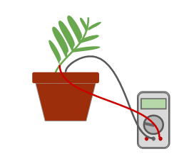
We then had to acquire our data. We placed 2 electrodes on our Mimosa, one in its soil as a reference and one on the node of the branch stimulated.

After that, we connected it to a voltmeter and tested our protocol. That was when we encountered our first difficulty: the electrode would detach each time the plant was stimulated!
We thought about other types of electrodes, but they would've broken our stems and we didn't want to hurt our Mimosa. We were quite stumped.

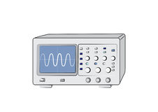
That is when we had an idea: why not use an oscilloscope! The oscilloscope’s electrodes are easy to place and with their hook-like shape wouldn't fall of!

We found our physics teacher and asked him if he could lend us an oscilloscope and its electrodes. He did more than that! He showed us many types of electrodes, helping us choose the most adapted, and helped us install the oscilloscope, showing us how to set it up, how to acquire the data directly on a USB key (instead of filming the screen and try to transform it into data) and testing its usefulness on Mimosa with us.

Thanks to this new tool we were able to design our final precise protocol that we will use to acquire data. So we repeated a simple experience for all the conditions that we described above. Indeed we created a mechanical stimulus during an electrical tension acquisition with the oscilloscope to observe the response on the drawn graph.

We knew that amplitude of the signal after the stimulus and the time it takes to go back to “normal” (return time) were two good indicators to quantify the response. So, as you might expect it, we measured both for each of our 27 graphs.

What are our results?

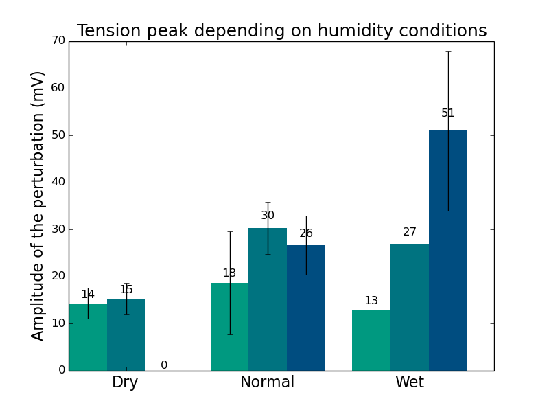
Then, we decided to plot the averages values per plant (repetitions) as one bar but the different plants (replicates) separately. Thus we obtained those two graphs (the first one represents the amplitude of the signal’s peak and the second one the return time, both depending on water conditions).

In both case, we seem to see an increase of both the amplitude of the perturbation and the return time as we expected. This finding would mean that water would have a direct impact on the electric response of the plant.

But this trend, is not measurable. Indeed we have been constrained to name the conditions “arbitrary” because our soil humidity sensor appeared to be unworking.    

Anyway, we have also notices that in each case, the return time and the amplitude of the peak are directly correlated. Indeed we can see exactly the same relative differences between all the replicates on the two graphs.

   

Finally, this project was for us a chance to develop our background knowledge on a particular subject and to train our project leading skills. Hopefully, it might brings you [readers] something on one of this two aspects of research!

Curious? Interested? Want to know more? Have a look at the links :

• Want to read scientific articles about Mimosa pudica and its thigmonastic reaction? Have a look here or there!
• If you want more information, but easier to understand than scientific articles, you might prefer reading this, that and what about this instead!
• Or maybe you want to grow out your own Mimosa pudica? You can find information here!

Does Escherichia coli respond to a nutrient gradient ?

 @EColorRace

On this final Biosensor week, we focused on the very known model microorganism Escherichia coli, the bacteria who lives in the lower intestines of humans and mammals. This bacteria is largely used in microbiology as it is the simplest organism to study complex mechanisms. They have a flagella that allow them to move in order to reach food. Food of bacteria is actually all nutrients like sugar, alcohol or amino acids that they need to develop and make some colonies. Depending on the nutrients available, their growth can be affected. There exists many different strains of E.coli, and fluorescent ones particularly interest us. Fluorescence might be useful to distinguish two strains of bacteria by naked eyes, by observing colonies of different colors! They can be stained with a fluorescent dye, in order to produce fluorescent images through UV lamp. As we were very interested in motility, fluorescence and growth of this bacteria, our main question was :

Who between starving E. coli and satiated ones is more sensitive to a nutrient gradient ?

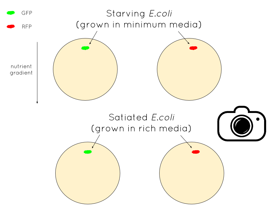
To answer this question we compared the speed of starving and satiated bacteria. We used two different strains, one marked with a green fluorescent protein (GFP, see how a nobel prize discovered it here!) and another marked with a red fluorescent protein (RFP). Starving bacteria are grown in a minimum media  for more than one night so that they have the nutrients strictly necessary to survive. Satiated bacteria are grown in a rich media with more nutrients than the absolutely necessary ones.

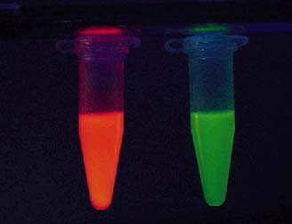
To produce the nutrient gradient through the petri dish  we tilled plates half full of media with food so that nutrients would be more concentrated on one side. Then we filled it with water and agar so bacteria can “swim” on it and look for food.                             Figure1. RFP and GFP

 

The experimental set-up consist in placing starving and satiated bacteria on the no food side of the plate and take picture for 24 hours of their moves toward food.

Who’s going to win the race?

Figure2. Experimental set-up

To collect data, we designed an electronical device that takes photo every 10 minutes in order to see bacteria moving. Of course we could not take picture ourselves as their movement take a while and we should have stand for more than 12h in the lab ! To realize that device, we used a stepper motor. On the top of it we placed a huge plexi plate carve with cutter laser so that 2O petri dishes can stand without falling. This device permit the petri dishes to be  just under the camera for the time laps at a defined time.

Figure3. A new lab robot

But as it always happen in science, we had some troubles. The stepper motor was not strong enough to carry the plate and our bacteria in minimum media died…

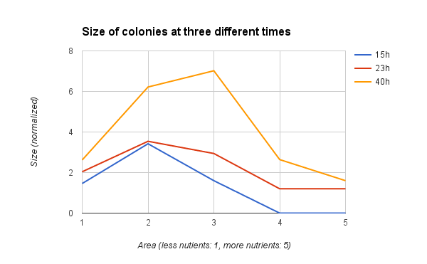
We decided to estimate the response to a gradient of nutriment of a single strain of E. coli, the red ones, for three different times (bottom right side of Figure2). The times were 15h after putting the bacteria on the plate, 23h and 40h.  Our new problematic is indeed :

How RFP respond to a nutrient gradient over time ?

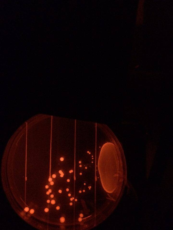
The protocol remain the same but the analysis is different. Instead of measuring speed we decided to focus on three parameters indicating a response to the gradient: the number of colonies formed, their size and the area they grew in. We divided each plate in five areas. One is where there is less nutrients and five correspond to the most concentrated region.

T1 = 15h            T2 = 23h        T3 = 40h

Figure4. Our new analysis set-up

You can see on this graph that the number of colonies globally increases over time. More interesting, there are more and more colonies on the areas where nutrients are more concentrated, especially areas 2 and 3 but even 4 after more hours (23h). It means that some E. coli moved from their starting point to develop a colony in a more conducive environment to grow. To know more about bacteria moves, look at this video!

You can see on this second graph that the size of bacteria also globally increases over time (red curve above blue and orange curve above red). Furthermore, colonies seem to be bigger in areas with more nutrient (area 3) after a long period such as  40h (orange curve).

Regarding those results, we can conclude that bacteria respond to a nutrient gradient through time and actually feel it. We also observe that when there is enough food in the area, they stop moving and form bigger colonies beside going farther toward food. But we can expect that after a long period, number and size of colonies will be maximum in area 5.

Thus, we proved that bacteria feel a gradient of food and go through it!

You can read this scientific article (1) to know more about how motile bacteria grow on heterogeneous surface.

We now have to do this experiment again with starving bacteria to answer our first question. But a perspective would be to study interactions between the two considered strains and organize a rate between them. This time they are on the same plate and competed for food. This experiment should demonstrate that E.coli interact and so have a group effect on each other.

Reference:

• Koster, D., Mayo, A., Bren, A. and Alon, U. (2012). Surface Growth of a Motile Bacterial Population Resembles Growth in a Chemostat. Journal of Molecular Biology, 424(3-4), pp.180-191.
• Pubs.acs.org, (2016). A Simple Method for GFP- and RFP-based Dual Color Single-Molecule Localization Microscopy - ACS Chemical Biology (ACS Publications). [online] Available at: http://pubs.acs.org/doi/abs/10.1021/acschembio.5b00046 [Accessed 12 Feb. 2016].
• Kearns, D. (2010). A field guide to bacterial swarming motility. Nature Reviews Microbiology, 8(9), pp.634-644.

You can follow us on twitter:   https://twitter.com/EColorRace?lang=fr